Problem Statement
A project is represented as a directed, acyclic graph G(V, E) where the nodes in the graph correspond to task and the arcs in the graph specify precedence relationships between the tasks. Arc (u, v) appears in the graph mean task u must be completed prior to performing task v (Fig. 1).
Two dummy tasks could be added, the first one represents the start processing of the project and is a predecessor of every other task, while final one denotes the end of project's processing and is the successor of every other task.
Each task can be defined by its duration, start and finish dates.
After started, any task cannot be stopped or delayed.
Each task requires a constant number of units of a renewable resource. The objective of RCPSP is to complete the project as soon as possible without violating any constraints, in other
MS-RCPSP Problem Formulation As a practical extension of RCPSP, MS-RCPSP adds the skills domain of the resources and aim to minimize the makespan. At a time only one resource can be assigned to a given task, in other words, any resource can not handle more than one tasks concurrently. Each task requires a subset of skills while each resource own an other unique sub-set of skills, therefore not every resource could handle a given task. MS-RCPSP can be conceptually formulated based on the following notations:
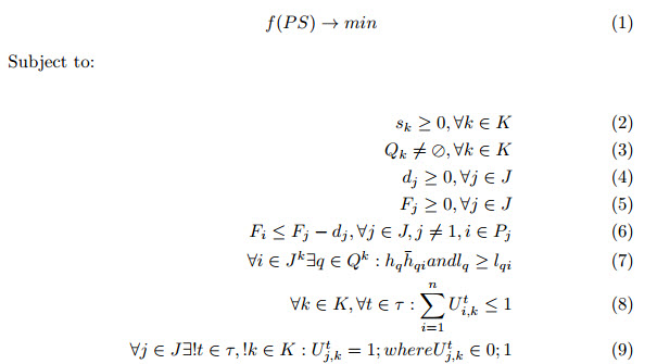
The feasible project schedule (PS) consists of J = 1,.., n tasks and K = 1,..., m resources. The cost of performing task j by resource k is ckj = dj * sk. For simplicity, we have modified the cost of the task’s performance from ckj to cj, because only one resource can be assigned to given task in the duration of the project. Hence, there is no need to distinguish various costs for the same task. Formally, MS-RCPSP could be regarded as mimization problem as follows:
Each solution (i.e. schedule) is represented by a vector of elements, the number of elements (i.e. the size of vector) equal to the number of tasks. The value of each ele-ment demonstrates the resource which executes the corresponding task.
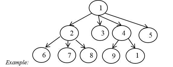
Fig. 1. The relationship between tasks
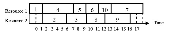
Fig. 2. A feasible project schedule
Fig. 1 demonstrates the relationship between tasks, based on that task 9 could not be started until task 4 finished, while task 6 and task 8 could be executed simultane-ously.
Fig. 2 depicts a feasible project schedule where:
- Set of task J={1, 2, 3, 4, 5, 6, 7, 8, 9, 10}
- Set of resource K={1, 2}.
The duration of tasks can be represented as follows:
| Task | 1 | 2 | 3 | 4 | 5 | 6 | 7 | 8 | 9 | 10 |
| Duration | 2 | 4 | 3 | 5 | 2 | 2 | 5 | 3 | 4 | 2 |
The schedule depicted in Fig. 2 can be represented as follows:
| Task | 1 | 2 | 3 | 4 | 5 | 6 | 7 | 8 | 9 | 10 |
| Resouce | 1 | 2 | 2 | 1 | 1 | 1 | 1 | 2 | 2 | 1 |
The above vector show that, the resource 1 is responsible for executing tasks 1, 4, 5, 6, 10 while the resource 2 handles the rest one.
Measurement model
The original Cuckoo Search algorithm is designed to deal with the floating point value data, while MS-RCPSP’s solution are the array of integer value elements. Thus we build a new measurement model in order to measure the difference between two schedules (i.e. solutions) as follow.
- Unit vector P = (p1, p2, ... pn); pi = 100/(ki-1) where ki is the number of resources that could handle task Ti.
- The difference between two schedules X =(x1, x2, ... xn) and Y=(y1, y2, ... yn) is the differential vector D =(d1, d2, ... dn);
D = X-Y
- The sum of the schedule Y and differential vector D is schedules X =(x1, x2, ... xn) where
- xi = possition(round (yi + di));
- possition(i): the resource which corresponding to the position i
Where:
-
di = pi . (order (xi) - order(yi) );
-
order (xi): the position of the resource (xi) in the Ki
Example:
Assume that there are 6 resources could handle task T1: K1 = ={R1, R3, R4, R5, R9, R10}. Thus: k1 = 6; p1 = 100/(6-1) = 20
Assume that there are 5 resources could handle task T2: K2 = {R3, R5, R7, R8, R10 }. Thus: k2 = 5; p2 = 100/(5-1) = 25
| Order | 0 | 1 | 2 | 3 | 4 | 5 |
| Resource | R1 | R3 | R4 | R5 | R9 | R10 |
| Resource | R3 | R5 | R7 | R8 | R10 |
Consider 2 schedules: X = (3,5); Y =(5,10);
| Schedule\Task | T1 | T2 |
| X | R3 | R5 |
| Y | R5 | R10 |
D = X-Y =(d1, d2)
Where:
- d1 = p1 . abs (order (x1) - order(y1) ) = 20. abs(1-3) =40
- d2 = p2 . abs (order (x2) - order(y2) ) = 25. abs(1-4) =75
Thus D =(40,75).
Consider D’=(35.71, 5.23)
We have Z = X+D’= (5,8)
| Task | T1 | T2 |
| X | R3 | R5 |
| D’ | 35.71 | 5.23 |
| pi. order(xi) | 20 | 60 |
| X+D’ | 55.71 | 65.23 |
| Z= X+D’ | R5 | R8 |